There are many different classifications of probability distributions. Some of them include the normal distribution, chi square distribution, binomial distribution, and Poisson distribution. The different probability distributions serve different purposes and represent different data generation processes.
The distribution of a statistical data set (or a population) is a listing or function showing all the possible values (or intervals) of the data and how often they occur. When a distribution of categorical data is organized, you see the number or percentage of individuals in each group.
A probability distribution is a statistical function that describes all the possible values and likelihoods that a random variable can take within a given range. These factors include the distribution's mean (average), standard deviation, skewness, and kurtosis.
General Properties of Probability Distributions
p(x) = the likelihood that random variable takes a specific value of x. The sum of all probabilities for all possible values must equal 1. Furthermore, the probability for a particular value or range of values must be between 0 and 1.Similar to mean and variance, other moments give useful information about random variables. The moment generating function (MGF) of a random variable X is a function MX(s) defined as MX(s)=E[esX]. We say that MGF of X exists, if there exists a positive constant a such that MX(s) is finite for all s∈[−a,a].
A probability distribution for a particular random variable is a function or table of values that maps the outcomes in the sample space to the probabilities of those outcomes. For example, in an experiment of tossing a coin twice, the sample space is. {HH, HT, TH, TT}.
The cumulative distribution function (FX) gives the probability that the random variable X is less than or equal to a certain amount x. Its formula is: Summing the values for all outcomes less than or equal to x will give the solution.
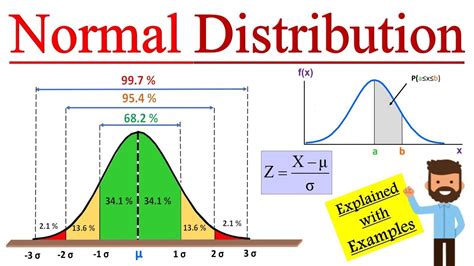
The cumulative distribution function of the standard normal distribution, denoted by Φ(z), represents the probability that the standard normal variable Z is less than or equal to the value z — that is, Pr{Z ≤ z}.
The (cumulative) distribution function of a random variable X, evaluated at x, is the probability that X will take a value less than or equal to x. You simply let the mean and variance of your random variable be 0 and 1, respectively. This is called standardizing the normal distribution.
The whole "probability can never be greater than 1" applies to the value of the CDF at any point. This means that the integral of the PDF over any interval must be less than or equal to 1. A: The PDF at x is greater than 1. Remember that there is no area under a point, meaning there is no probability under a point.
Specifically, we can compute the probability that a discrete random variable equals a specific value (probability mass function) and the probability that a random variable is less than or equal to a specific value (cumulative distribution function).
Cumulative Frequency Plots. A cumulative frequency plot is a way to display cumulative information graphically. It shows the number, percentage, or proportion of observations that are less than or equal to particular values.
A discrete random variable is a variable that represents numbers found by counting. For example: number of marbles in a jar, number of students present or number of heads when tossing two coins. A probability distribution has all the possible values of the random variable and the associated probabilities.
Normalpdf finds the probability of getting a value at a single point on a normal curve given any mean and standard deviation. Normalcdf just finds the probability of getting a value in a range of values on a normal curve given any mean and standard deviation.
Thus, we should be able to find the
CDF and
PDF of Y. It is usually more straightforward to start from the
CDF and then to find the
PDF by taking the derivative of the
CDF.
Let X be a Uniform(0,1) random variable, and let Y=eX.
- Find the CDF of Y.
- Find the PDF of Y.
- Find EY.
Remember that P(x<X≤x+Δ)=FX(x+Δ)−FX(x). =dFX(x)dx=F′X(x),if FX(x) is differentiable at x. is called the probability density function (PDF) of X.
Use the CDF to determine the probability that a random observation that is taken from the population will be less than or equal to a certain value. You can also use this information to determine the probability that an observation will be greater than a certain value, or between two values.
The Normal Distribution functions:
#1: normalpdf pdf = Probability Density Function. This function returns the probability of a single value of the random variable x. Use this to graph a normal curve. Using this function returns the y-coordinates of the normal curve. Syntax: normalpdf (x, mean, standard deviation)For example, if you were tossing a coin to see how many heads you were going to get, if the coin landed on heads that would be a “success.” The difference between the two functions is that one (BinomPDF) is for a single number (for example, three tosses of a coin), while the other (BinomCDF) is a cumulative probability
Probability Density Functions (PDF):
A PDF is simply the derivative of a CDF. Thus a PDF is also a function of a random variable, x, and its magnitude will be some indication of the relative likelihood of measuring a particular value.